Python Charts with matplotlib: Bar Charts, Line Charts and a Report Dashboard

A table of numbers answers questions for anyone with time to read it. A good chart answers them in two seconds. In this lesson you'll turn the sales analysis from lessons 11 and 13 into a visual dashboard with matplotlib, Python's most widely used charting library and the foundation many others are built on.

Which chart do you need?

Before writing code, decide which question you're answering. Almost every business chart falls into one of these four:

Setup and your first chart

pip install matplotlib pandas

(Activate your virtual environment first, as in lesson 10.) The basic matplotlib pattern never changes: create a figure with one or more "axes" (each axes is one chart), draw, then save or show it.

import matplotlib.pyplot as plt

months = ["Jan", "Feb", "Mar"]
sales = [3887.5, 2525.0, 3765.0]

fig, ax = plt.subplots(figsize=(7, 4))   # size in inches
ax.plot(months, sales, marker="o")
ax.set_title("Sales by month")
ax.set_ylabel("Revenue ($)")
fig.savefig("sales_by_month.png", dpi=150)   # save the image
plt.show()                                   # open a window (Jupyter shows it automatically)

Always work with fig and ax (the "object-oriented interface"). You'll see code online that calls plt.plot() directly: it works for quick charts but gets messy as soon as you want more than one.

Preparing the data with pandas

We start from the sales file. As you know from lesson 11, one row has no region; it belongs to Maria, who covers the Midwest:

import pandas as pd

df = pd.read_csv("sales.csv", parse_dates=["date"])
df["region"] = df["region"].fillna("Midwest")
df["revenue"] = df["units"] * df["price"]

by_region = df.groupby("region")["revenue"].sum().sort_values()
print(by_region)

region
East       2707.5
Midwest    2870.0
West       4600.0
Name: revenue, dtype: float64

Bar charts: comparing categories

fig, ax = plt.subplots(figsize=(7, 4))
ax.barh(by_region.index, by_region.values, color="#2f6fed")
ax.set_title("West leads Q1 2026 sales")
ax.set_xlabel("Revenue ($)")

for i, v in enumerate(by_region.values):          # label each bar with its value
    ax.text(v, i, f" ${v:,.0f}", va="center")

ax.spines[["top", "right"]].set_visible(False)     # remove unnecessary borders
fig.tight_layout()
fig.savefig("sales_by_region.png", dpi=150)

Three decisions make this chart easier to read: horizontal bars (long names fit without rotating them), bars sorted from smallest to largest (with sort_values(), the biggest ends up on top) and the value written next to each bar, so nobody has to estimate it from the axis.

Plotting straight from pandas

DataFrames and Series have a .plot() method that uses matplotlib under the hood. It's ideal for pivot tables:

months = {1: "Jan", 2: "Feb", 3: "Mar"}

by_product = df.pivot_table(index=df["date"].dt.month, columns="product",
                            values="revenue", aggfunc="sum", fill_value=0)
by_product.index = by_product.index.map(months)
print(by_product)

ax = by_product.plot(kind="bar", stacked=True, rot=0, figsize=(7, 4))
ax.set_title("Sales by product and month")

product  Chocolate  Coffee     Tea
date
Jan            0.0  3080.0   807.5
Feb          640.0   840.0  1045.0
Mar          880.0  2030.0   855.0

kind accepts "line", "bar", "barh", "hist", "box", "scatter" and more. The dictionary gives us short, predictable month labels that don't depend on your computer's language settings.

A dashboard with several charts

With plt.subplots(1, 3) you get three axes in a row and fill them one by one:

months = {1: "Jan", 2: "Feb", 3: "Mar"}
by_month = df.groupby(df["date"].dt.month)["revenue"].sum()
by_month.index = by_month.index.map(months)

fig, axs = plt.subplots(1, 3, figsize=(15, 4.5))

axs[0].plot(by_month.index, by_month.values, marker="o", linewidth=2)
axs[0].set_title("Sales by month")
axs[0].set_ylim(bottom=0)

by_product.plot(kind="bar", stacked=True, ax=axs[1], rot=0)
axs[1].set_title("Sales by product")
axs[1].set_xlabel("")
axs[1].legend(title="", frameon=False)

axs[2].barh(by_region.index, by_region.values, color="#2f6fed")
axs[2].set_title("Sales by region")

for ax in axs:
    ax.spines[["top", "right"]].set_visible(False)

fig.suptitle("Sales dashboard · Q1 2026", fontsize=14, fontweight="bold")
fig.tight_layout()
fig.savefig("sales_dashboard.png", dpi=150)

The result:

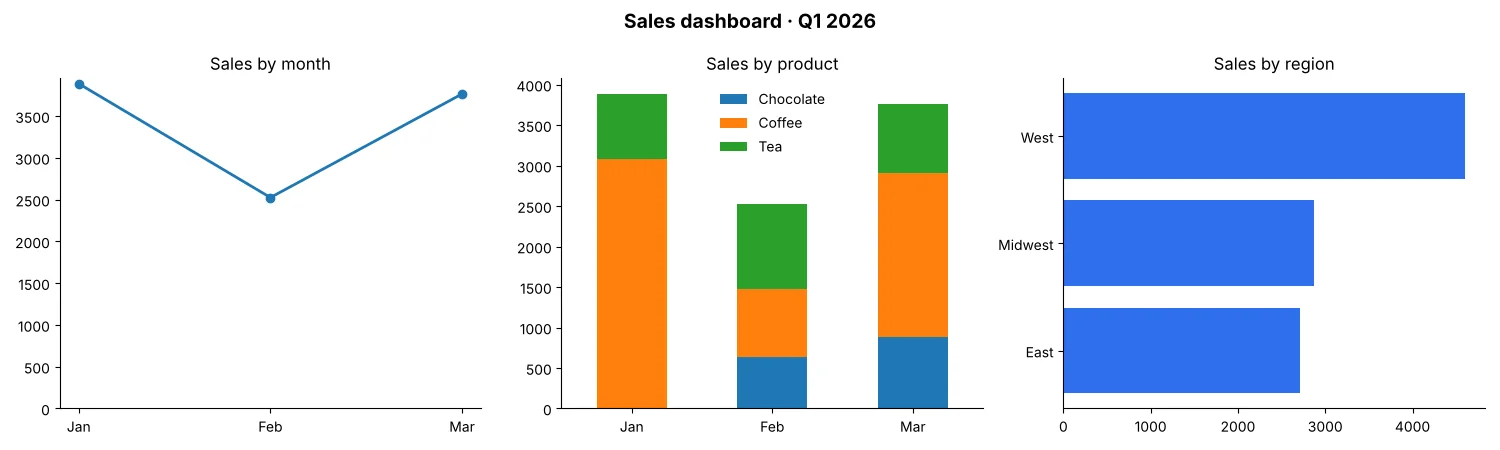
The two-second read: February was the weak month (mostly because coffee dropped from $3,080 to $840), chocolate starts selling in February, and the West alone brings in 45.2% of the quarter's $10,177.50. That's exactly what a good dashboard should deliver.

Charts that don't mislead

Real case: does heat sell ice cream?

The owner of an ice cream shop in Myrtle Beach, South Carolina, suspects she sells more on hot days and wants to decide how much mix to prepare based on the forecast. For 10 days she wrote down the high temperature and the cones sold. To see whether two numeric variables are related, the right chart is a scatter plot: one dot per day.

import matplotlib.pyplot as plt
import pandas as pd

# Ice cream shop in Myrtle Beach, SC: high temperature and cones sold over 10 days
data = pd.DataFrame({
    "temperature": [76, 79, 80, 82, 84, 86, 88, 90, 92, 94],
    "cones":       [118, 135, 150, 149, 170, 182, 190, 214, 220, 241],
})
r = data["temperature"].corr(data["cones"])
hot = data[data["temperature"] > 86]["cones"].mean()
mild = data[data["temperature"] <= 86]["cones"].mean()
print(f"Correlation: {r:.2f}")
print(f"Average above 86°F: {hot:.0f} cones")
print(f"Average at 86°F or below: {mild:.0f} cones")

fig, ax = plt.subplots(figsize=(6, 4))
ax.scatter(data["temperature"], data["cones"], color="#2459d6", s=60)
ax.set_title(f"Hotter days, more ice cream (correlation {r:.2f})")
ax.set_xlabel("High temperature (°F)")
ax.set_ylabel("Cones sold")
ax.set_ylim(bottom=0)
ax.spines[["top", "right"]].set_visible(False)
fig.tight_layout()
fig.savefig("heat_ice_cream.png", dpi=150)

Correlation: 0.99
Average above 86°F: 216 cones
Average at 86°F or below: 151 cones

Correlation runs from −1 to 1: near 1, the two variables rise together; near 0, there's no linear relationship. The practical takeaway is clear: days above 86°F sell an average of 216 cones versus 151, about 65 more. But careful: correlation isn't causation. If those hot days were also weekends or the Fourth of July, part of the jump could come from that. In lesson 16 you'll see how a model learns relationships like this to make predictions.

Common matplotlib errors

The most frequent error appears when two lists aren't the same length, for example three months and four values:

ValueError: x and y must have same first dimension, but have shapes (3,) and (4,)

The "shapes" (3,) and (4,) are the lengths of each list: a month is missing or there's an extra value. Other common stumbles:

import matplotlib.pyplot as plt
import pandas as pd

e = pd.read_csv("expenses.csv", parse_dates=["date"])
by_cat = e.groupby("category")["amount"].sum().sort_values()
by_month = e.groupby(e["date"].dt.to_period("M"))["amount"].sum()
by_month.index = by_month.index.astype(str)       # "2026-09", "2026-10"…

fig, axs = plt.subplots(1, 2, figsize=(12, 4))

axs[0].barh(by_cat.index, by_cat.values, color="#2f6fed")
for i, v in enumerate(by_cat.values):
    axs[0].text(v, i, f" ${v:,.0f}", va="center")
axs[0].set_title("Food is 42% of spending")

axs[1].plot(by_month.index, by_month.values, marker="o")
axs[1].set_ylim(bottom=0)
axs[1].set_title("Spending by month")

for ax in axs:
    ax.spines[["top", "right"]].set_visible(False)

fig.tight_layout()
fig.savefig("expense_dashboard.png", dpi=150)

Summary

• The basic pattern: fig, ax = plt.subplots(), draw on ax, then fig.savefig().
• Lines for time, sorted bars to compare categories, stacked bars for composition, scatter plots for relationships.
• pandas plots directly with .plot(kind=...), and you can combine both styles by passing ax=.
• A dashboard is one figure with several axes: plt.subplots(rows, columns).
• Bars start at zero, one message per chart, few colors and no 3D.

Next lesson: Web Scraping with Python: requests and BeautifulSoup Step by Step. You'll collect data that doesn't come in any file by extracting it from web pages, responsibly.